Trajectory¶

In the module pyinduct.trajectory are some trajectory generators defined. Besides you can find here a trivial (constant) input signal generator as well as input signal generator for equilibrium to equilibrium transitions for hyperbolic and parabolic systems.

class ConstantTrajectory(const=0)[source]¶

Bases: pyinduct.simulation.SimulationInput

Trivial trajectory generator for a constant value as simulation input signal.

Parameters:	const (numbers.Number) – Desired constant value of the output.

class FlatString(y0, y1, z0, z1, t0, dt, params)[source]¶

Bases: pyinduct.simulation.SimulationInput

Class that implements a flatness based control approach for the “string with mass” model.

class InterpTrajectory(t, u, show_plot=False)[source]¶

Bases: pyinduct.simulation.SimulationInput

Provides a system input through one-dimensional linear interpolation between the given vectors $u$ and $t$ .

Parameters:	t (array_like) – Vector $t$ with time steps. u (array_like) – Vector $u$ with function values, corresponding to the vector $t$ . show_plot (boolean) – A plot window with plot(t, u) will pop up if it is true.

get_plot()[source]¶

class RadTrajectory(l, T, param_original, bound_cond_type, actuation_type, n=80, sigma=1.1, K=2.0, show_plot=False)[source]¶

Bases: pyinduct.trajectory.InterpTrajectory

Class that implements a flatness based control approach for the reaction-advection-diffusion equation

$\dot x(z,t) = a_2 x''(z,t) + a_1 x'(z,t) + a_0 x(z,t)$

with the boundary condition

bound_cond_type == "dirichlet": $x(0,t)=0$

A transition from $x'(0,0)=0$ to $x'(0,T)=1$ is considered.

With $x'(0,t) = y(t)$ where $y(t)$ is the flat output.

bound_cond_type == "robin": $x'(0,t) = \alpha x(0,t)$

A transition from $x(0,0)=0$ to $x(0,T)=1$ is considered.

With $x(0,t) = y(t)$ where $y(t)$ is the flat output.

and the actuation

actuation_type == "dirichlet": $x(l,t)=u(t)$

actuation_type == "robin": $x'(l,t) = -\beta x(l,t) + u(t)$ .

The flat output $y(t)$ will calculated with gevrey_tanh().

class SignalGenerator(waveform, t, scale=1, offset=0, **kwargs)[source]¶

Bases: pyinduct.trajectory.InterpTrajectory

Signal generator that combines scipy.signal.waveforms and InterpTrajectory.

Parameters:

waveform (str) – A waveform which is provided from scipy.signal.waveforms.
t (array_like) – Array with time steps or pyinduct.simulation.Domain instance.
scale (numbers.Number) – Scale factor: output = waveform_output*scale + offset.
offset (numbers.Number) – Offset value: output = waveform_output*scale + offset.
kwargs – The corresponding keyword arguments to the desired scipy.signal waveform. In addition to the kwargs of the desired waveform function from scipy.signal (which will simply forwarded) the keyword arguments frequency (for waveforms: ‘sawtooth’ and ‘square’) and phase_shift (for all waveforms) provided.

class SmoothTransition(states, interval, method, differential_order=0)[source]¶

Bases: object

A smooth transition between two given steady-states states on an interval using either: polynomial method trigonometric method

To create smooth transitions.

Parameters:	states (tuple) – States at beginning and end of interval. interval (tuple) – Time interval. method (str) – Method to use (`poly` or `tanh`). differential_order (int) – Grade of differential flatness $\gamma$ .

coefficient_recursion(c0, c1, param)[source]¶

Return to the recursion

$c_k(t) = \frac{ \dot c_{k-2}(t) - a_1 c_{k-1}(t) - a_0 c_{k-2}(t) }{ a_2 }$

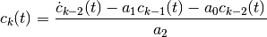
with initial values

$c_0 = numpy.array([c_0^{(0)}, ... , c_0^{(N)}]) \\ c_1 = numpy.array([c_1^{(0)}, ... , c_1^{(N)}])$

as much as computable subsequent coefficients

$c_2 = numpy.array&([c_2^{(0)}, ... , c_2^{(N-1)}]) \\ c_3 = numpy.array&([c_3^{(0)}, ... , c_3^{(N-1)}]) \\ &\vdots \\ c_{2N-1} = numpy.array&([c_{2N-1}^{(0)}]) \\ c_{2N} = numpy.array&([c_{2N}^{(0)}])$

Parameters:	c0 (array_like) – $c_0$ c1 (array_like) – $c_1$ param (array_like) – (a_2, a_1, a_0, None, None)
Returns:	$C = \{0: c_0, 1: c_1, ..., 2N-1: c_{2N-1}, 2N: c_{2N}\}$
Return type:	dict

gevrey_tanh(T, n, sigma=1.1, K=2.0)[source]¶

Provide Gevrey function

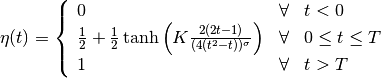
$\eta(t) = \left\{ \begin{array}{lcl} 0 & \forall & t<0 \\ \frac{1}{2} + \frac{1}{2}\tanh \left(K \frac{2(2t-1)}{(4(t^2-t))^\sigma} \right) & \forall & 0\le t \le T \\ 1 & \forall & t>T \end{array} \right.$

with the Gevrey-order $\rho=1+\frac{1}{\sigma}$ and the derivatives up to order n.

Note

For details of the recursive calculation of the derivatives see:

Rudolph, J., J. Winkler und F. Woittennek: Flatness Based Control of Distributed Parameter Systems: Examples and Computer Exercises from Various Technological Domains (Berichte aus der Steuerungs- und Regelungstechnik). Shaker Verlag GmbH, Germany, 2003.

Parameters:	T (numbers.Number) – End of the time domain=[0,T]. n (int) – The derivatives will calculated up to order n. sigma (numbers.Number) – Constant $\sigma$ to adjust the Gevrey order $\rho=1+\frac{1}{\sigma}$ of $\varphi(t)$ . K (numbers.Number) – Constant to adust the slope of $\varphi(t)$ .
Returns:	(numpy.array([[ $\varphi(t)$ ], ... ,[ $\varphi^{(n)}(t)$ ]]), numpy.array([0,...,T])
Return type:	tuple

power_series(z, t, C, spatial_der_order=0, temporal_der_order=0)[source]¶

Compute the function values

$x^{(j,i)}(z,t)=\sum_{k=0}^{N} c_{k+j}^{(i)}(t) \frac{z^k}{k!}.$

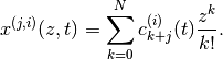
Parameters:	z (array_like) – Spatial steps to compute. t (array like) – Temporal steps to compute. C (dict) – Coeffient dictionary which keys correspond to the coefficient index. The values are 2D numpy.array’s. For example C[1] should provide a 2d-array with the coefficient $c_1(t)$ and at least $i$ temporal derivatives $\text{np.array}([c_1^{(0)}(t), ... , c_1^{(i)}(t)]).$ spatial_der_order (int) – Spatial derivative order $j$ . temporal_der_order (int) – Temporal derivative order $i$ .
Returns:	Array of shape (len(t), len(z)).
Return type:	numpy.array

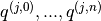
temporal_derived_power_series(z, C, up_to_order, series_termination_index, spatial_der_order=0)[source]¶

Compute the temporal derivatives

$q^{(j,i)}(z=z^*,t) = \sum_{k=0}^{N} \underbrace{c_{k+j}^{(i)}}_{\text{C[k+j][i,:]}} \frac{{z^*}^k}{k!}, \qquad i=0,...,n.$

Parameters:

z (numbers.Number) – Evaluation point $z^*$ .
C (dict) –
Coeffient dictionary which keys correspond to the coefficient index. The values are 2D numpy.array’s. For example C[1] should provide a 2d-array with the coefficient $c_1(t)$ and at least $n$ temporal derivatives

$\text{np.array}([c_1^{(0)}(t), ... , c_1^{(i)}(t)]).$
up_to_order (int) – Max. temporal derivative order $n$ to compute.
series_termination_index (int) – Series termination index $N$ .
spatial_der_order (int) – Spatial derivativ order $j$ .

Returns:

numpy.array( [ $q^{(j,0)}, ... , q^{(j,n)}$ ] )