R.a.d. eq. with dirichlet b.c. (fem approximation)¶

Reaction-advection-diffusion equation with dirichlet boundary condition by $z=0$ and dirichlet actuation by $z=l$ .

$\begin{align*} \dot{x}(z,t) = a_2x''&(z,t) + a_1x'(z,t) + a_0x(z,t) && z\in (0, l), t>0\\ x(z,0) &= x_0(z) && z\in [0,l]\\ x(0,t) &= 0 && t>0\\ x(l,t) &= u(t) && t>0 \end{align*}$

example: heat equation
- $a_2=1,\quad a_1= 0, \quad a_0=0, \quad x_0(z)=0$
- $u(t)$ –> pyinduct.trajectory.RadTrajectory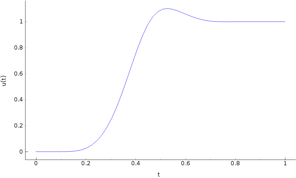
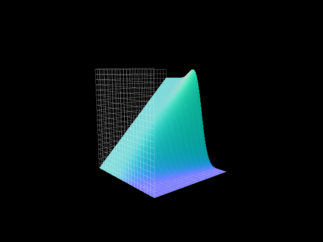
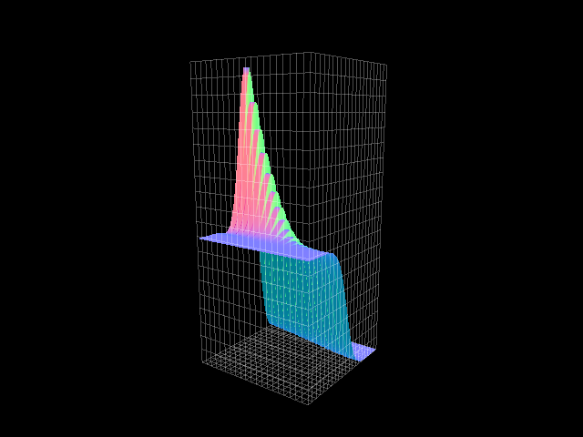
- $x(z,t)$
- $x'(z,t)$
- corresponding 3d plots

$x(z,t)$	$x'(z,t)$

with:
- inital functions $\varphi_1(z),...,\varphi_{n+1}(z)$
- test functions $\varphi_1(z),...,\varphi_n(z)$
- where the functions $\varphi_1(z),..,\varphi_n(z)$ met the homogeneous b.c.
  
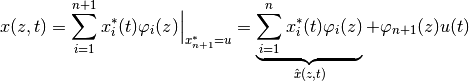
  $\varphi_1(l),..,\varphi_n(l)=\varphi_1(0),..,\varphi_n(0)=0$
- only $\varphi_{n+1}$ can draw the actuation
- functions $\varphi_1(z),...,\varphi_{n+1}(z)$ e.g. from type pyinduct.shapefunctions.LagrangeFirstOrder or pyinduct.shapefunctions.LagrangeSecondOrder, see pyinduct.shapefunctions
approach:

$x(z,t) = \sum_{i=1}^{n+1} x_i^*(t) \varphi_i(z)\Big|_{x^*_{n+1}=u} = \underbrace{\sum_{i=1}^{n} x_i^*(t) \varphi_i(z)}_{\hat x(z,t)} + \varphi_{n+1}(z) u(t)$

weak formulation...

$\begin{align*} \langle\dot{x}(z,t),\varphi_j(z)\rangle &= a_2 \langle x''(z,t),\varphi_j(z)\rangle \\ &\hphantom =+ a_1 \langle x'(z,t), \varphi_j(z)\rangle + a_0 \langle x(z,t), \varphi_j(z)\rangle && j=1,...,n \end{align*}$

... and derivation shift to work with lagrange 1st order initial functions

$\begin{align*} \langle\dot{x}(z,t),\varphi_j(z)\rangle &= \overbrace{[a_2 [x'(z,t)\varphi_j(z)]_0^l}^{=0} - a_2 \langle x'(z,t),\varphi'_j(z)\rangle \\ &\hphantom =+ a_1 \langle x'(z,t), \varphi_j(z)\rangle + a_0 \langle x(z,t), \varphi_j(z)\rangle && j=1,...,n \\ \langle\dot{\hat{x}}(z,t),\varphi_j(z)\rangle + \langle\varphi_{N+1}(z),\varphi_j(z)\rangle \dot u(t) &= - a_2 \langle \hat x'(z,t),\varphi'_j(z)\rangle - a_2 \langle \varphi'_{N+1}(z),\varphi'_j(z)\rangle u(t) \\ &\hphantom =+ a_1 \langle \hat x'(z,t), \varphi_j(z)\rangle + a_1 \langle \varphi'_{N+1}(z), \varphi_j(z)\rangle u(t) + \\ &\hphantom =+ a_0 \langle \hat x(z,t), \varphi_j(z)\rangle + a_0 \langle \varphi_{N+1}(z), \varphi_j(z)\rangle u(t) && j=1,...,n \end{align*}$

leads to state space model for the weights $\boldsymbol{x}^*=(x_1^*,...,x_n^*)^T$ :

$\begin{align*} \dot{\boldsymbol{x}}^*(t) = A \boldsymbol x^*(t) + \boldsymbol b_0 u(t) + \boldsymbol b_1 \dot{u}(t) \end{align*}$

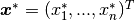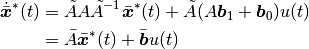
input derivative elimination through the transformation:
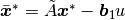
- $\bar{\boldsymbol{x}}^* = \tilde A \boldsymbol x^* - \boldsymbol{b}_1 u$
- $\text{e.g.: } \tilde A = I$
- leads to

$\begin{align*} \dot{\bar{\boldsymbol{x}}}^*(t) &= \tilde A A\tilde A^{-1} \bar{\boldsymbol{x}}^*(t) + \tilde A(A\boldsymbol b_1 + \boldsymbol b_0) u(t) \\ &= \bar A \bar{\boldsymbol{x}}^*(t) +\bar{\boldsymbol{b}} u(t) \end{align*}$

source code:

import pyinduct.trajectory as tr
import pyinduct.core as cr
import pyinduct.shapefunctions as sh
import pyinduct.simulation as sim
import pyinduct.visualization as vis
import pyinduct.placeholder as ph
from pyinduct import register_base, get_base

import numpy as np
import pyqtgraph as pg

n_fem = 17
T = 1
l = 1
param = [1, 0, 0, None, None]  # or try this: param = [1, -0.5, -8, None, None]     :)))
a2, a1, a0, _, _ = param

temp_domain = sim.Domain(bounds=(0, T), num=1e2)
spat_domain = sim.Domain(bounds=(0, l), num=n_fem * 11)

# initial and test functions
nodes, fem_funcs = sh.cure_interval(sh.LagrangeFirstOrder, spat_domain.bounds, node_count=n_fem)
act_fem_func = fem_funcs[-1]
not_act_fem_funcs = fem_funcs[1:-1]
vis_fems_funcs = fem_funcs[1:]
register_base("act_func", act_fem_func)
register_base("sim", not_act_fem_funcs)
register_base("vis", vis_fems_funcs)

# trajectory
u = tr.RadTrajectory(l, T, param, "dirichlet", "dirichlet")

# weak form ...
x = ph.FieldVariable("sim")
phi = ph.TestFunction("sim")
act_phi = ph.ScalarFunction("act_func")
not_acuated_weak_form = sim.WeakFormulation([
    # ... of the homogeneous part of the system
    ph.IntegralTerm(ph.Product(x.derive(temp_order=1), phi), limits=spat_domain.bounds),
    ph.IntegralTerm(ph.Product(x.derive(spat_order=1), phi.derive(1)), limits=spat_domain.bounds, scale=a2),
    ph.IntegralTerm(ph.Product(x.derive(spat_order=1), phi), limits=spat_domain.bounds, scale=-a1),
    ph.IntegralTerm(ph.Product(x, phi), limits=spat_domain.bounds, scale=-a0),
    # ... of the inhomogeneous part of the system
    ph.IntegralTerm(ph.Product(ph.Product(act_phi, phi), ph.Input(u, order=1)), limits=spat_domain.bounds),
    ph.IntegralTerm(
        ph.Product(ph.Product(act_phi.derive(1), phi.derive(1)), ph.Input(u)), limits=spat_domain.bounds, scale=a2),
    ph.IntegralTerm(ph.Product(ph.Product(act_phi.derive(1), phi), ph.Input(u)), limits=spat_domain.bounds, scale=-a1),
    ph.IntegralTerm(ph.Product(ph.Product(act_phi, phi), ph.Input(u)), limits=spat_domain.bounds, scale=-a0)
])

# system matrices \dot x = A x + b0 u + b1 \dot u
cf = sim.parse_weak_formulation(not_acuated_weak_form)
E1_inv = cf.inverse_e_n
ss = cf.convert_to_state_space()
A = ss.A[1]
b0 = np.array(np.matrix(ss.B[1][:, 0]).T)
b1 = np.array(np.matrix(ss.B[1][:, 1]).T)

# transformation
A_tilde = np.diag(np.ones(A.shape[0]), 0)
A_bar = np.dot(np.dot(A_tilde, A), np.linalg.inv(A_tilde))
b_bar = np.dot(A_tilde, np.dot(A, b1) + b0)

# simulation
start_func = cr.Function(lambda z: 0)
start_state = np.array([sim.project_on_base(start_func, get_base(cf.weights, 0))]).flatten()
transf_start_state = np.dot(A_tilde, start_state) - (b1 * u(time=0)).flatten()
ss = sim.StateSpace("transf_sim", A_bar, b_bar, input_handle=u)
sim_temp_domain, sim_transf_weights = sim.simulate_state_space(ss, transf_start_state, temp_domain)

# back-transformation
u_vec = np.matrix(u.get_results(sim_temp_domain)).T
sim_weights = np.nan * np.zeros((sim_transf_weights.shape[0], len(not_act_fem_funcs)))
for i in range(sim_transf_weights.shape[0]):
    sim_weights[i, :] = np.dot(np.linalg.inv(A_tilde), sim_transf_weights[i, :]) + (b1 * u_vec[i]).flatten()

# visualisation
save_pics = False
vis_weights = np.hstack((np.matrix(sim_weights), u_vec))
eval_d = sim.evaluate_approximation("vis", vis_weights, sim_temp_domain, spat_domain, spat_order=0)
der_eval_d = sim.evaluate_approximation("vis", vis_weights, sim_temp_domain, spat_domain, spat_order=1)
win1 = vis.PgAnimatedPlot(eval_d, labels=dict(left='x(z,t)', bottom='z'), save_pics=save_pics)
win2 = vis.PgAnimatedPlot(der_eval_d, labels=dict(left='x\'(z,t)', bottom='z'), save_pics=save_pics)
win3 = vis.PgSurfacePlot(eval_d, title="x(z,t)")
win4 = vis.PgSurfacePlot(der_eval_d, title="x'(z,t)")

# save pics
if save_pics:
    path = vis.save_2d_pg_plot(u.get_plot(), 'rad_dirichlet_traj')[1]
    win3.gl_widget.grabFrameBuffer().save(path + 'rad_dirichlet_3d_x.png')
    win4.gl_widget.grabFrameBuffer().save(path + 'rad_dirichlet_3d_dx.png')
pg.QtGui.QApplication.instance().exec_()