String with mass system: simulation, controller and observer implementation
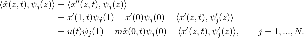
This script (swm_observer.py) shows how to simulate a distributed system with pyinduct, using the string with mass example, which is illustrated in figure 5 and can described by the pde

and the boundary conditions

where the deflection of the string is described by the field variable  .
The partial derivatives of
.
The partial derivatives of  w.r.t. time
  and space
  are denoted by means of dots
and primes, respectively. On the boundary by
are denoted by means of dots
and primes, respectively. On the boundary by  the mass
  is fixed at the string and on the
boundary by
is fixed at the string and on the
boundary by  the deflection of the string can changed by use of the force (input variable)
  .
.
Furthermore the flatness based controller and observer implementation is shown by this example. The design of the controller and the observer is obtained from the paper
- [Woi2012]: Frank Woittennek. „Beobachterbasierte Zustandsrückführungen für hyperbolische verteiltparametrische Systeme“.In: Automatisierungstechnik 60.8 (2012).
The control law (equation 29) and the observer (equation 41) from [Woi2012] were simply tipped off. You can find
the implementation in the functions build_control_law() and build_observer_can().
-
build_system_state_space(approx_label, u, params)[source]¶ The boundary conditions can considered through integration by parts of the weak formulation:
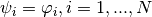
The field variable is approximated with the functions
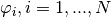 which are registered
under the label approx_label
which are registered
under the label approx_label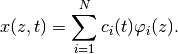
In order to derive a numerical scheme the galerkin method is used, meaning
 .
.Parameters: - approx_label (string) – Shapefunction label for approximation.
- u (
pyinduct.simulation.SimulationInput) – Input variable - params – Python class with the member m (mass).
Returns: State space model
Return type: limits = (0, 1) x = ph.FieldVariable(approx_label) psi = ph.TestFunction(approx_label) wf = sim.WeakFormulation( [ ph.IntegralTerm(ph.Product(x.derive(temp_order=2), psi), limits=limits), ph.IntegralTerm(ph.Product(x.derive(spat_order=1), psi.derive(1)), limits=limits), ph.ScalarTerm(ph.Product(x(0).derive(temp_order=2), psi(0)), scale=params.m), ph.ScalarTerm(ph.Product(ph.Input(u), psi(1)), scale=-1), ], name="swm_system" ) return sim.parse_weak_formulation(wf).convert_to_state_space()
-
build_control_law(approx_label, params)[source]¶ The control law from [Woi2012] (equation 29)
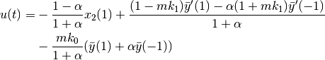
is simply tipped off in this function, whereas
![\begin{align*}
\bar{y}(\theta) &= \left\{\begin{array}{lll}
\xi_1 + m(1-e^{-\theta/m})\xi_2 +
\int_0^\theta (1-e^{-(\theta-\tau)/m}) (x_1'(\tau) + x_2(\tau)) \, dz
& \forall & \theta\in[-1, 0) \\
\xi_1 + m(e^{\theta/m}-1)\xi_2 +
\int_0^\theta (e^{(\theta-\tau)/m}-1) (x_1'(-\tau) - x_2(-\tau)) \, dz
& \forall & \theta\in[0, 1]
\end{array}\right. \\
\bar{y}'(\theta) &= \left\{\begin{array}{lll}
e^{-\theta/m}\xi_2 + \frac{1}{m}
\int_0^\theta e^{-(\theta-\tau)/m} (x_1'(\tau) + x_2(\tau)) \, dz
& \forall & \theta\in[-1, 0) \\
e^{\theta/m}\xi_2 + \frac{1}{m}
\int_0^\theta e^{(\theta-\tau)/m} (x_1'(-\tau) - x_2(-\tau)) \, dz
& \forall & \theta\in[0, 1].
\end{array}\right.
\end{align*}](../_images/math/4e78c10a4ae6f3fbd648b95afe550e49af706763.png)
Parameters: - approx_label (string) – Shapefunction label for approximation.
- params –
Python class with the members:
- m (mass)
- k1_ct, k2_ct, alpha_ct (controller parameters)
Returns: Control law
Return type: x = ph.FieldVariable(approx_label) dz_x1 = x.derive(spat_order=1) x2 = x.derive(temp_order=1) xi1 = x(0) xi2 = x(0).derive(temp_order=1) scalar_scale_funcs = [cr.Function(lambda theta: params.m * (1 - np.exp(-theta / params.m))), cr.Function(lambda theta: params.m * (-1 + np.exp(theta / params.m))), cr.Function(lambda theta: np.exp(-theta / params.m)), cr.Function(lambda theta: np.exp(theta / params.m))] register_base("int_scale1", cr.Function(lambda tau: 1 - np.exp(-(1 - tau) / params.m))) register_base("int_scale2", cr.Function(lambda tau: -1 + np.exp((-1 + tau) / params.m))) register_base("int_scale3", cr.Function(lambda tau: np.exp(-(1 - tau) / params.m) / params.m)) register_base("int_scale4", cr.Function(lambda tau: np.exp((-1 + tau) / params.m) / params.m)) limits = (0, 1) y_bar_plus1 = [ph.ScalarTerm(xi1), ph.ScalarTerm(xi2, scale=scalar_scale_funcs[0](1)), ph.IntegralTerm(ph.Product(ph.ScalarFunction("int_scale1"), dz_x1), limits=limits), ph.IntegralTerm(ph.Product(ph.ScalarFunction("int_scale1"), x2), limits=limits)] y_bar_minus1 = [ph.ScalarTerm(xi1), ph.ScalarTerm(xi2, scale=scalar_scale_funcs[1](-1)), ph.IntegralTerm(ph.Product(ph.ScalarFunction("int_scale2"), dz_x1), limits=limits, scale=-1), ph.IntegralTerm(ph.Product(ph.ScalarFunction("int_scale2"), x2), limits=limits)] dz_y_bar_plus1 = [ph.ScalarTerm(xi2, scale=scalar_scale_funcs[2](1)), ph.IntegralTerm(ph.Product(ph.ScalarFunction("int_scale3"), dz_x1), limits=limits), ph.IntegralTerm(ph.Product(ph.ScalarFunction("int_scale3"), x2), limits=limits)] dz_y_bar_minus1 = [ph.ScalarTerm(xi2, scale=scalar_scale_funcs[3](-1)), ph.IntegralTerm(ph.Product(ph.ScalarFunction("int_scale4"), dz_x1), limits=limits, scale=-1), ph.IntegralTerm(ph.Product(ph.ScalarFunction("int_scale4"), x2), limits=limits)] return sim.FeedbackLaw(ut.scale_equation_term_list( [ph.ScalarTerm(x2(1), scale=-(1 - params.alpha_ct))] + ut.scale_equation_term_list(dz_y_bar_plus1, factor=(1 - params.m * params.k1_ct)) + ut.scale_equation_term_list(dz_y_bar_minus1, factor=-params.alpha_ct * (1 + params.m * params.k1_ct)) + ut.scale_equation_term_list(y_bar_plus1, factor=-params.m * params.k0_ct) + ut.scale_equation_term_list(y_bar_minus1, factor=-params.alpha_ct * params.m * params.k0_ct), factor=(1 + params.alpha_ct) ** -1 ))
-
build_observer_can(sys_approx_label, obs_approx_label, sys_input, params)[source]¶ The observer from [Woi2012] (equation 41)
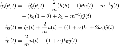
is simply tipped off in this function. The boundary condition (equation 41d)

is considered through integration by parts of the term
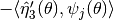 from the weak formulation of equation 41a:
Parameters: - sys_approx_label (string) – Shapefunction label for system approximation.
- obs_approx_label (string) – Shapefunction label for observer approximation.
- sys_input (
pyinduct.simulation.SimulationInput) – Input variable - params –
Python class with the members:
- m (mass)
- k1_ob, k2_ob, alpha_ob (observer parameters)
Returns: Observer
Return type: limits = (-1, 1) def heavi(z): return 0 if z < 0 else (0.5 if z == 0 else 1) register_base("obs_scale1", cr.Function(lambda z: -2 / params.m * (heavi(z) - 1) * z, domain=limits)) register_base("obs_scale2", cr.Function(lambda z: -(params.k0_ob * (1 - z) + params.k1_ob - 1 / params.m), domain=limits)) obs_scale1 = ph.ScalarFunction("obs_scale1") obs_scale2 = ph.ScalarFunction("obs_scale2") def dummy_one(z): return 1 register_base("eta1", cr.Function(dummy_one, domain=limits)) register_base("eta2", cr.Function(dummy_one, domain=limits)) eta1 = ph.FieldVariable("eta1") eta2 = ph.FieldVariable("eta2") eta3 = ph.FieldVariable(obs_approx_label) psi = ph.TestFunction(obs_approx_label) obs_err = sim.ObserverError(sim.FeedbackLaw([ ph.ScalarTerm(ph.FieldVariable(sys_approx_label, location=0), scale=-1) ]), sim.FeedbackLaw([ ph.ScalarTerm(eta3(-1).derive(spat_order=1), scale=-params.m / 2), ph.ScalarTerm(eta3(1).derive(spat_order=1), scale=-params.m / 2), ph.ScalarTerm(eta1(0), scale=-params.m / 2), ]), weighted_initial_error=0.1) u_vec = sim.SimulationInputVector([sys_input, obs_err]) d_eta1 = sim.WeakFormulation( [ ph.ScalarTerm(eta1(0).derive(temp_order=1), scale=-1), ph.ScalarTerm(ph.Input(u_vec, index=0), scale=2 / params.m), ph.ScalarTerm(ph.Input(u_vec, index=1), scale=-(1 + params.alpha_ob) * params.k0_ob) ], dynamic_weights="eta1" ) d_eta2 = sim.WeakFormulation( [ ph.ScalarTerm(eta2(0).derive(temp_order=1), scale=-1), # index error in paper ph.ScalarTerm(eta1(0)), ph.ScalarTerm(ph.Input(u_vec, index=0), scale=2 / params.m), ph.ScalarTerm(ph.Input(u_vec, index=1), scale=-(1 + params.alpha_ob) * params.k1_ob - 2 * params.k0_ob) ], dynamic_weights="eta2" ) d_eta3 = sim.WeakFormulation( [ ph.IntegralTerm(ph.Product(eta3.derive(temp_order=1), psi), limits=limits, scale=-1), # sign error in paper ph.IntegralTerm(ph.Product(ph.Product(obs_scale1, psi), ph.Input(u_vec, index=0)), limits=limits, scale=-1), ph.IntegralTerm(ph.Product(ph.Product(obs_scale2, psi), ph.Input(u_vec, index=1)), limits=limits), # \hat y ph.IntegralTerm(ph.Product(eta3(-1).derive(spat_order=1), psi), limits=limits, scale=1 / 2), ph.IntegralTerm(ph.Product(eta3(1).derive(spat_order=1), psi), limits=limits, scale=1 / 2), ph.IntegralTerm(ph.Product(eta1, psi), limits=limits, scale=1 / 2), # shift ph.IntegralTerm(ph.Product(eta3, psi.derive(1)), limits=limits), ph.ScalarTerm(ph.Product(eta3(1), psi(1)), scale=-1), # bc ph.ScalarTerm(ph.Product(psi(-1), eta2(0))), ph.ScalarTerm(ph.Product(ph.Input(u_vec, index=1), psi(-1)), scale=1 - params.alpha_ob), # bc \hat y ph.ScalarTerm(ph.Product(eta3(-1).derive(spat_order=1), psi(-1)), params.m / 2), ph.ScalarTerm(ph.Product(eta3(1).derive(spat_order=1), psi(-1)), params.m / 2), ph.ScalarTerm(ph.Product(eta1(1), psi(-1)), params.m / 2), ], dynamic_weights=obs_approx_label ) d_eta1_cfs = sim.parse_weak_formulation(d_eta1) d_eta2_cfs = sim.parse_weak_formulation(d_eta2) d_eta3_cfs = sim.parse_weak_formulation(d_eta3) obs_ss = sim.convert_cfs_to_state_space([d_eta1_cfs, d_eta2_cfs, d_eta3_cfs]) return sim.build_observer_from_state_space(obs_ss)
- script:
import pyinduct.trajectory as tr
import pyinduct.core as cr
import pyinduct.shapefunctions as sh
import pyinduct.simulation as sim
import pyinduct.visualization as vis
import pyinduct.placeholder as ph
import pyinduct.utils as ut
from pyinduct import register_base
import numpy as np
import matplotlib.pyplot as plt
import pyqtgraph as pg
.
.
.
if __name__ == "__main__":

    # which observer
    nf_observer = True

    # temporal and spatial domain specification
    t_end = 8
    temp_domain = sim.Domain(bounds=(0, t_end), step=.01)
    spat_domain = sim.Domain(bounds=(0, 1), step=.01)

    # system/simulation parameters
    params = Parameters
    params.node_count = 10
    params.m = 1.0
    params.tau = 1.0  # hard written to 1 in this example script
    params.sigma = 1.0  # hard written to 1 in this example script

    # controller parameters
    params.k0_ct = 10
    params.k1_ct = 10
    params.alpha_ct = 0

    # controller parameters
    params.k0_ob = 10
    params.k1_ob = 10
    params.alpha_ob = 0

    # initial function
    sys_nodes, sys_funcs = sh.cure_interval(sh.LagrangeNthOrder, spat_domain.bounds, node_count=10, order=1)
    ctrl_nodes, ctrl_funcs = sh.cure_interval(sh.LagrangeNthOrder, spat_domain.bounds, node_count=20, order=1)
    register_base("sim", sys_funcs)
    register_base("ctrl", ctrl_funcs)
    if nf_observer:
        obs_can_nodes, obs_can_funcs = sh.cure_interval(sh.LagrangeNthOrder, (-1, 1), node_count=25, order=4)
        register_base("obs_can", obs_can_funcs)
    else:
        obs_org_nodes1, obs_org_funcs1 = sh.cure_interval(sh.LagrangeNthOrder, spat_domain.bounds, node_count=9,
                                                          order=2)
        obs_org_nodes2, obs_org_funcs2 = sh.cure_interval(sh.LagrangeNthOrder, spat_domain.bounds, node_count=9,
                                                          order=2)
        register_base("x1_hat", obs_org_funcs1)
        register_base("x2_hat", obs_org_funcs1)

    # system input
    if 1:
        # trajectory for the new input (closed_loop_traj)
        smooth_transition = tr.SmoothTransition((0, 1), (2, 4), method="poly", differential_order=2)
        closed_loop_traj = SecondOrderFeedForward(smooth_transition, params)
        # controller
        ctrl = sim.Feedback(build_control_law("ctrl", params))
        u = sim.SimulationInputSum([closed_loop_traj, ctrl])
    else:
        # trajectory for the original input (open_loop_traj)
        open_loop_traj = tr.FlatString(y0=0, y1=1, z0=spat_domain.bounds[0], z1=spat_domain.bounds[1],
                                       t0=1, dt=3, params=params)
        # u = sim.SimulationInputSum([open_loop_traj])
        u = sim.SimulationInputSum([tr.ConstantTrajectory(0)])

    # system state space
    sys_ss = build_system_state_space("sim", spat_domain.bounds, u, params)
    sys_init = np.zeros(sys_ss.A[1].shape[0])
    # sys_init = np.hstack((np.ones(sys_funcs.shape[0]), np.zeros(sys_funcs.shape[0])))

    # observer state space
    if nf_observer:
        obs_ss = build_observer_can("sim", "obs_can", u, params)
        obs_init = np.ones(obs_ss.A[1].shape[0])
    else:
        obs_ss = build_observer_org("sim", "x1_hat", "x2_hat", u, params)
        # obs_init = np.zeros(obs_ss.A[1].shape[0])
        obs_init = np.hstack((np.ones(obs_org_funcs1.shape[0]), np.zeros(obs_org_funcs2.shape[0])))

    # simulation
    if nf_observer:
        sim_domain, x_w, eta1_w, eta2_w, eta3_w = sim.simulate_state_space(
            sys_ss, sys_init, temp_domain, obs_ss=obs_ss, obs_init_state=obs_init
        )
    else:
        sim_domain, x_w, x1_w, x2_w = sim.simulate_state_space(
            sys_ss, sys_init, temp_domain, obs_ss=obs_ss, obs_init_state=obs_init
        )

    # evaluate data
    x_data = sim.process_sim_data("sim", x_w, temp_domain, spat_domain, 0, 0)[0]
    if nf_observer:
        eta1_data = sim.process_sim_data("eta1", eta1_w, sim_domain, sim.Domain(bounds=(0, 1), num=1e1), 0, 0)[0]
        dz_et3_m1_0 = sim.process_sim_data("obs_can", eta3_w, sim_domain, sim.Domain(bounds=(-1, 0), num=1e1), 0, 1)[1]
        dz_et3_0_p1 = sim.process_sim_data("obs_can", eta3_w, sim_domain, sim.Domain(bounds=(0, 1), num=1e1), 0, 1)[1]
        x_obs_data = vis.EvalData(eta1_data.input_data, -params.m / 2 * (
            dz_et3_m1_0.output_data + np.fliplr(dz_et3_0_p1.output_data) + eta1_data.output_data
        ))
    else:
        x_obs_data = sim.process_sim_data("x1_hat", x1_w, sim_domain, sim.Domain(bounds=(0, 1), num=1e1), 0, 0)[0]

    # animation
    plot1 = vis.PgAnimatedPlot([x_data, x_obs_data])
    plot2 = vis.PgSurfacePlot(x_data)
    plot3 = vis.PgSurfacePlot(x_obs_data)
    pg.QtGui.QApplication.instance().exec_()
    vis.MplSlicePlot([x_data, x_obs_data], spatial_point=0)
    plt.show()