Simulation¶

Simulation infrastructure with helpers and data structures for preprocessing of the given equations and functions for postprocessing of simulation data.

class SimulationInput(name='')[source]¶

Bases: object

Base class for all objects that want to act as an input for the time-step simulation.

The calculated values for each time-step are stored in internal memory and can be accessed by get_results() (after the simulation is finished).

Note

Due to the underlying solver, this handle may get called with time arguments, that lie outside of the specified integration domain. This should not be a problem for a feedback controller but might cause problems for a feedforward or trajectory implementation.

clear_cache()[source]¶

Clear the internal value storage.

When the same SimulationInput is used to perform various simulations, there is no possibility to distinguish between the different runs when get_results() gets called. Therefore this method can be used to clear the cache.

get_results(time_steps, result_key='output', interpolation='nearest', as_eval_data=False)[source]¶

Return results from internal storage for given time steps.

Raises:	`Error` – If calling this method before a simulation was run.
Parameters:	time_steps – Time points where values are demanded. result_key – Type of values to be returned. interpolation – Interpolation method to use if demanded time-steps are not covered by the storage, see `scipy.interpolate.interp1d()` for all possibilities. as_eval_data (bool) – Return results as `EvalData` object for straightforward display.
Returns:	Corresponding function values to the given time steps.

class SimulationInputSum(inputs)[source]¶

Bases: pyinduct.simulation.SimulationInput

Helper that represents a signal mixer.

class WeakFormulation(terms, name, dominant_lbl=None)[source]¶

Bases: object

This class represents the weak formulation of a spatial problem. It can be initialized with several terms (see children of EquationTerm). The equation is interpreted as

$term_0 + term_1 + ... + term_N = 0.$

Parameters:	terms (list) – List of object(s) of type EquationTerm. name (string) – Name of this weak form. dominant_lbl (string) – Name of the variable that dominates this weak form.

parse_weak_formulation(weak_form, finalize=False)[source]¶

Parses a WeakFormulation that has been derived by projecting a partial differential equation an a set of test-functions. Within this process, the separating approximation $x^n(z, t) = \sum_{i=1}^n c_i^n(t) \varphi_i^n(z)$ is plugged into the equation and the separated spatial terms are evaluated, leading to a ordinary equation system for the weights $c_i^n(t)$ .

Parameters:	weak_form – Weak formulation of the pde. finalize (bool) – Default: False. If you have already defined the dominant labels of the weak formulations you can set this to True. See `CanonicalEquation.finalize()`
Returns:	The spatially approximated equation in a canonical form.
Return type:	`CanonicalEquation`

create_state_space(canonical_equations)[source]¶

Create a state-space system constituted by several CanonicalEquations (created by parse_weak_formulation())

Parameters:	canonical_equations – List of `CanonicalEquation`’s.
Raises:	`ValueError` – If compatibility criteria cannot be fulfilled
Returns:	State-space representation of the approximated system
Return type:	`StateSpace`

class StateSpace(a_matrices, b_matrices, base_lbl=None, input_handle=None, c_matrix=None, d_matrix=None)[source]¶

Bases: object

Wrapper class that represents the state space form of a dynamic system where

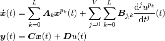
$\boldsymbol{\dot{x}}(t) &= \sum\limits_{k=0}^{L}\boldsymbol{A}_{k} \boldsymbol{x}^{p_k}(t) + \sum\limits_{j=0}^{V} \sum\limits_{k=0}^{L}\boldsymbol{B}_{j, k} \frac{\mathrm{d}^j u^{p_k}}{\mathrm{d}t^j}(t) \\ \boldsymbol{y}(t) &= \boldsymbol{C}\boldsymbol{x}(t) + \boldsymbol{D}u(t)$

which has been approximated by projection on a base given by weight_label.

Parameters:

a_matrices (dict) – State transition matrices $\boldsymbol{A}_{p_k}$ for the corresponding powers of $\boldsymbol{x}$
b_matrices (dict) – Cascaded dictionary for the input matrices $\boldsymbol{B}_{j, k}$ in the sequence: temporal derivative order, exponent .
input_handle – function handle, returning the system input $u(t)$
c_matrix – $\boldsymbol{C}$
d_matrix – $\boldsymbol{D}$

rhs(_t, _q)[source]¶

Callback for the integration of the dynamic system, described by this object.

Parameters:	_t (float) – timestamp _q (array) – weight vector
Returns:	$\boldsymbol{\dot{x}}(t)$
Return type:	(array)

simulate_state_space(state_space, initial_state, temp_domain, settings=None)[source]¶

Wrapper to simulate a system given in state space form:

$\dot{q} = A_pq^p + A_{p-1}q^{p-1} + \dotsb + A_0q + Bu.$

Parameters:	state_space (`StateSpace`) – State space formulation of the system. initial_state – Initial state vector of the system. temp_domain (`Domain`) – Temporal domain object. settings (dict) – Parameters to pass to the `set_integrator()` method of the `scipy.ode` class, with the integrator name included under the key `name`.
Returns:	Time `Domain` object and weights matrix.
Return type:	tuple

simulate_system(weak_form, initial_states, temporal_domain, spatial_domain, derivative_orders=(0, 0), settings=None)[source]¶

Convenience wrapper for simulate_systems().

Parameters:

weak_form (WeakFormulation) – Weak formulation of the system to simulate.
initial_states (numpy.ndarray) – Array of core.Functions for $x(t=0, z), \dot{x}(t=0, z), \dotsc, x^{(n)}(t=0, z)$ .
temporal_domain (Domain) – Domain object holding information for time evaluation.
spatial_domain (Domain) – Domain object holding information for spatial evaluation.
derivative_orders (tuple) – tuples of derivative orders (time, spat) that shall be evaluated additionally as values
settings – Integrator settings, see simulate_state_space().

simulate_systems(weak_forms, initial_states, temporal_domain, spatial_domains, derivative_orders=None, settings=None)[source]¶

Convenience wrapper that encapsulates the whole simulation process.

Parameters:

weak_forms ((list of) WeakFormulation) – (list of) Weak formulation(s) of the system(s) to simulate.
initial_states (dict, numpy.ndarray) – Array of core.Functions for $x(t=0, z), \dot{x}(t=0, z), \dotsc, x^{(n)}(t=0, z)$ .
temporal_domain (Domain) – Domain object holding information for time evaluation.
spatial_domains (dict) – Dict with Domain objects holding information for spatial evaluation.
derivative_orders (dict) – Dict, containing tuples of derivative orders (time, spat) that shall be evaluated additionally as values
settings – Integrator settings, see simulate_state_space().

Note

The name attributes of the given weak forms must be unique!

Returns:	List of `EvalData` objects, holding the results for the FieldVariable and demanded derivatives.
Return type:	list

get_sim_result(weight_lbl, q, temp_domain, spat_domain, temp_order, spat_order, name='')[source]¶

Create handles and evaluate at given points.

Parameters:

weight_lbl (str) – Label of Basis for reconstruction.
temp_order – Order or temporal derivatives to evaluate additionally.
spat_order – Order or spatial derivatives to evaluate additionally.
q – weights
spat_domain (Domain) – Domain object providing values for spatial evaluation.
temp_domain (Domain) – Time steps on which rows of q are given.
name (str) – Name of the WeakForm, used to generate the data set.

evaluate_approximation(base_label, weights, temp_domain, spat_domain, spat_order=0, name='')[source]¶

Evaluate an approximation given by weights and functions at the points given in spatial and temporal steps.

Parameters:	weights – 2d np.ndarray where axis 1 is the weight index and axis 0 the temporal index. base_label (str) – Functions to use for back-projection. temp_domain (`Domain`) – For steps to evaluate at. spat_domain (`Domain`) – For points to evaluate at (or in). spat_order – Spatial derivative order to use. name – Name to use.
Returns:	`EvalData`

parse_weak_formulations(weak_forms)[source]¶

Convenience wrapper for parse_weak_formulation().

Parameters:	weak_forms – List of `WeakFormulation`’s.
Returns:	List of `CanonicalEquation`’s.

get_sim_results(temp_domain, spat_domains, weights, state_space, names=None, derivative_orders=None)[source]¶

Convenience wrapper for get_sim_result().

Parameters:

temp_domain (Domain) – Time domain
spat_domains (dict) – Spatial domain from all subsystems which belongs to state_space as values and name of the systems as keys.
weights (numpy.array) – Weights gained through simulation. For example with simulate_state_space().
state_space (StateSpace) – Simulated state space instance.
names – List of names of the desired systems. If not given all available subssystems will be processed.
derivative_orders (dict) – Desired derivative orders.

Returns:

List of EvalData objects.

set_dominant_labels(canonical_equations, finalize=True)[source]¶

Set the dominant label (dominant_lbl) member of all given canonical equations and check if the problem formulation is valid (see background section: http://pyinduct.readthedocs.io/en/latest/).

If the dominant label of one or more CanonicalEquation is already defined, the function raise a UserWarning if the (pre)defined dominant label(s) are not valid.

Parameters:	canonical_equations – List of `CanonicalEquation` instances. finalize (bool) – Finalize the equations? Default: True.

class CanonicalEquation(name, dominant_lbl=None)[source]¶

Bases: object

Wrapper object, holding several entities of canonical forms for different weight-sets that form an equation when summed up. After instantiation, this object can be filled with information by passing the corresponding coefficients to add_to(). When the parsing process is completed and all coefficients have been collected, calling finalize() is required to compute all necessary information for further processing. When finalized, this object provides access to the dominant form of this equation.

Parameters:	name (str) – Unique identifier of this equation. dominant_lbl (str) – Label of the variable that dominates this equation.

add_to(weight_label, term, val, column=None)[source]¶

Add the provided val to the canonical form for weight_label, see CanonicalForm.add_to() for further information.

Parameters:	weight_label (str) – Basis to add onto. term – Coefficient to add onto, see `add_to()`. val – Values to add. column (int) – passed to `add_to()`.

dominant_form¶

direct access to the dominant CanonicalForm.

Note

finalize() must be called first.

Returns:	the dominant canonical form
Return type:	`CanonicalForm`

finalize()[source]¶: Finalize the Object. After the complete formulation has been parsed and all terms have been sorted into this Object via add_to() this function has to be called to inform this object about it. Furthermore, the f and G parts of the static_form will be copied to the dominant form for easier state-space transformation.

Note

This function must be called to use the dominant_form attribute.

finalize_dynamic_forms()[source]¶: Finalize all dynamic forms. See method CanonicalForm.finalize().

get_dynamic_terms()[source]¶

Returns:	Dictionary of terms for each weight set.
Return type:	dict

get_static_terms()[source]¶

Returns:	Terms that do not depend on a certain weight set.

input_function¶: The input handle for the equation.

static_form¶: WeakForm that does not depend on any weights. :return:

class CanonicalForm(name=None)[source]¶

Bases: object

The canonical form of an nth order ordinary differential equation system.

add_to(term, value, column=None)[source]¶

Adds the value value to term term. term is a dict that describes which coefficient matrix of the canonical form the value shall be added to.

Parameters:

term (dict) –
Targeted term in the canonical form h. It has to contain:
- name: Type of the coefficient matrix: ‘E’, ‘f’, or ‘G’.
- order: Temporal derivative order of the assigned weights.
- exponent: Exponent of the assigned weights.
value (numpy.ndarray) – Value to add.
column (int) – Add the value only to one column of term (useful if only one dimension of term is known).

convert_to_state_space()[source]¶

Convert the canonical ode system of order n a into an ode system of order 1.

Note

This will only work if the highest derivative order of the given form can be isolated. This is the case if the highest order is only present in one power and the equation system can therefore be solved for it.

Returns:
Return type:	`StateSpace` object

finalize()[source]¶: Finalizes the object. This method must be called after all terms have been added by add_to() and before convert_to_state_space() can be called. This functions makes sure that the formulation can be converted into state space form (highest time derivative only comes in one power) and collects information like highest derivative order, it’s power and the sizes of current and state-space state vector (dim_x resp. dim_xb). Furthermore, the coefficient matrix of the highest derivative order e_n_pb and it’s inverse are made accessible.

get_terms()[source]¶

Return all coefficient matrices of the canonical formulation.

Returns:	Structure: Type > Order > Exponent.
Return type:	Cascade of dictionaries

input_function¶