Eigenfunctions
This modules provides eigenfunctions for a certain set of second order spatial operators. Therefore functions for the computation of the corresponding eigenvalues are included. The functions which compute the eigenvalues are deliberately separated from the predefined eigenfunctions in order to handle transformations and reduce effort within the controller implementation.
-
class
SecondOrderOperator(a2=0, a1=0, a0=0, alpha1=0, alpha0=0, beta1=0, beta0=0, domain=(-inf, inf))[source]¶ Bases:
objectInterface class to collect all important parameters that describe a second order ordinary differential equation.
Parameters: - a2 (Number or callable) – coefficient
 .
. - a1 (Number or callable) – coefficient
 .
. - a0 (Number or callable) – coefficient
 .
. - alpha1 (Number) – coefficient
 .
. - alpha0 (Number) – coefficient
 .
. - beta1 (Number) – coefficient
 .
. - beta0 (Number) – coefficient
 .
.
-
get_adjoint_problem()[source]¶ Return the parameters of the operator
 describing the
the problem
describing the
the problem
where the
 are constant and whose boundary conditions
are given by
are constant and whose boundary conditions
are given by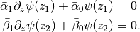
The following mapping is used:
Returns: Parameter set describing .Return type: SecondOrderOperator
- a2 (Number or callable) – coefficient
-
class
SecondOrderEigenVector(char_pair, coefficients, domain, derivative_order)[source]¶ Bases:
pyinduct.core.FunctionThis class provides eigenvectors of the form

of a linear second order spatial operator
 denoted by
where the
 are constant and whose boundary conditions are given
by
are constant and whose boundary conditions are given
by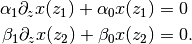
To calculate the corresponding eigenvectors, the problem
is solved for the eigenvalues
 , making use of the
characteristic roots
, making use of the
characteristic roots  given by
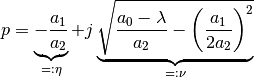
Note
To easily instantiate a set of eigenvectors for a certain system, use the
cure_hint()of this class or even better the helper-functioncure_interval().- Warn:
- Since an eigenvalue corresponds to a pair of conjugate complex characteristic roots, latter are only calculated for the positive half-plane since the can be mirrored. To obtain the orthonormal properties of the generated eigenvectors, the eigenvalue corresponding to the characteristic root 0+0j is ignored, since it leads to the zero function.
Parameters: - char_pair (tuple of complex) – Characteristic root, corresponding to the
eigenvalue for which the eigenvector is
to be determined.
(Can be obtained by
convert_to_characteristic_root()) - coefficients (tuple) – Constants of the exponential ansatz solution.
Returns: The eigenvector.
Return type: -
static
calculate_eigenvalues(domain, params, count, extended_output=False, **kwargs)[source]¶ Determine the eigenvalues of the problem given by parameters defined on domain .
Parameters: - domain (
Domain) – Domain of the spatial problem. - params (bunch-like) – Parameters of the system, see
__init__()for details on their definition. Long story short, it must contain .
. - count (int) – Amount of eigenvalues to generate.
- extended_output (bool) – If true, not only eigenvalues but also the corresponding characteristic roots and coefficients of the eigenvectors are returned. Defaults to False.
Keyword Arguments: debug (bool) – If provided, this parameter will cause several debug windows to open.
Returns: , ordered in increasing
order or tuple of ( )
if extended_output is True.
)
if extended_output is True.Return type: array or tuple of arrays
- domain (
-
static
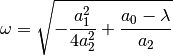
convert_to_characteristic_root(params, eigenvalue)[source]¶ Converts a given eigenvalue
into a
characteristic root by using the provided
parameters. The relation is given by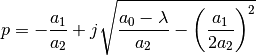
Parameters: - params (bunch) – system parameters, see
cure_hint(). - eigenvalue (real) – eigenvalue
Returns: characteristic root
Return type: complex number
- params (bunch) – system parameters, see
-
static
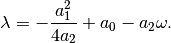
convert_to_eigenvalue(params, char_roots)[source]¶ Converts a pair of characteristic roots
 into an
eigenvalue by using the provided parameters.
The relation is given by
into an
eigenvalue by using the provided parameters.
The relation is given by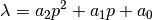
Parameters: - params (
SecondOrderOperator) – System parameters. - char_roots (tuple or array of tuples) – Characteristic roots
- params (
-
static
cure_hint(domain, params, count, derivative_order, **kwargs)[source]¶ Helper to cure an interval with eigenvectors.
Parameters: - domain (
Domain) – Domain of the spatial problem. - params (
SecondOrderOperator) – Parameters of the system, see__init__()for details on their definition. Long story short, it must contain .
. - count (int) – Amount of eigenvectors to generate.
- derivative_order (int) – Amount of derivative handles to provide.
- kwargs – will be passed to
calculate_eigenvalues()
Keyword Arguments: debug (bool) – If provided, this parameter will cause several debug windows to open.
Returns: An array holding the eigenvalues paired with a basis spanned by the eigenvectors.
Return type: tuple of (array,
Base)- domain (
-
class
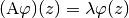
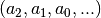
SecondOrderEigenfunction[source]¶ Bases:
objectWrapper for all eigenvalue problems of the form

with eigenfunctions
 and eigenvalues .
The roots of the characteristic equation (belonging to the ode) are denoted
by
and eigenvalues .
The roots of the characteristic equation (belonging to the ode) are denoted
by
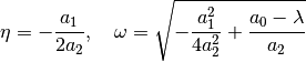
In the following the variable
 is called an eigenfrequency.
-
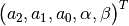
static
eigfreq_eigval_hint(param, l, n_roots)[source]¶ Parameters: - param (array_like) – Parameters
 .
. - l – End of the domain
![z\in[0, 1]](../_images/math/dae45b61dae56e0bd8fc7275407114b52153b824.png) .
. - n_roots (int) – Number of eigenfrequencies/eigenvalues to be compute.
Returns: Booth tuple elements are numpy.ndarrays of the same length, one for eigenfrequencies and one for eigenvalues.
![\Big(\big[\omega_1,...,\omega_\text{n\_roots}\Big],
\Big[\lambda_1,...,\lambda_\text{n\_roots}\big]\Big)](../_images/math/d8f5ce58efd7eca68255cb266f159f67c609d969.png)
Return type: tuple
- param (array_like) – Parameters
-
static
eigval_tf_eigfreq(param, eig_val=None, eig_freq=None)[source]¶ Provide corresponding of eigenvalues/eigenfrequencies for given eigenfreqeuncies/eigenvalues, depending on which type is given.
respectively
Parameters: - param (array_like) – Parameters .
- eig_val (array_like) – Eigenvalues .
- eig_freq (array_like) – Eigenfrequencies .
Returns: Eigenfrequencies
or eigenvalues
.Return type: numpy.array
- param (array_like) – Parameters
-
static
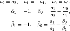
get_adjoint_problem(param)[source]¶ Return the parameters of the adjoint eigenvalue problem for the given parameter set. Hereby, dirichlet or robin boundary condition at


and dirichlet or robin boundary condition at


can be imposed.
Parameters: param (array_like) – To define a homogeneous dirichlet boundary condition set alpha or beta to None at the corresponding side. Possibilities:
 ,
, ,
,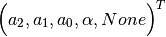 or
or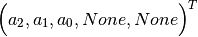 .
.
Returns: Parameters 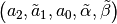 for
the adjoint problem
for
the adjoint problem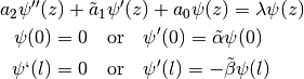
with
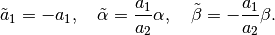
Return type: tuple
-
classmethod
solve_evp_hint(param, l, n=None, eig_val=None, eig_freq=None, max_order=2, scale=None)[source]¶ Provide the first n eigenvalues and eigenfunctions (wraped inside a pyinduct base). For the exact formulation of the considered eigenvalue problem, have a look at the docstring from the eigenfunction class from which you will call this method.
You must call this classmethod with one and only one of the kwargs:
- n (eig_val and eig_freq will be computed with the
eigfreq_eigval_hint()) - eig_val (eig_freq will be calculated with
eigval_tf_eigfreq()) - eig_freq (eig_val will be calculated with
eigval_tf_eigfreq()),
or (and) pass the kwarg scale (then n is set to len(scale)). If you have the kwargs eig_val and eig_freq already calculated then these are preferable, in the sense of performance.
Parameters: - param – Parameters
 see
evp_class.__doc__.
see
evp_class.__doc__. - l – End of the eigenfunction domain (start is 0).
- n – Number of eigenvalues/eigenfunctions to compute.
- eig_freq (array_like) – Pass your own choice of eigenfrequencies here.
- eig_val (array_like) – Pass your own choice of eigenvalues here.
- max_order – Maximum derivative order which must provided by the eigenfunctions.
- scale (array_like) – Here you can pass a list of values to scale the eigenfunctions.
Returns: Tuple with one list for the eigenvalues and one base which fractions are the eigenfunctions.
- n (eig_val and eig_freq will be computed with the
-
static
-
class
SecondOrderDirichletEigenfunction(om, param, l, scale=1, max_der_order=2)[source]¶ Bases:
pyinduct.eigenfunctions.LambdifiedSympyExpression,pyinduct.eigenfunctions.SecondOrderEigenfunctionThis class provides an eigenfunction
 to eigenvalue
problems of the form
to eigenvalue
problems of the form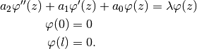
The eigenfrequency
must be provided (for example with the
eigfreq_eigval_hint()of this class).Parameters: - om (numbers.Number) – eigenfrequency
- param (array_like) –
- l (numbers.Number) – End of the domain
![z\in [0,l]](../_images/math/b0ae5f362d82201850219e2ff95dab8c02a55894.png) .
. - scale (numbers.Number) – Factor to scale the eigenfunctions.
- max_der_order (int) – Number of derivative handles that are needed.
-
static
eigfreq_eigval_hint(param, l, n_roots)[source]¶ Return the first n_roots eigenfrequencies
and
eigenvalues .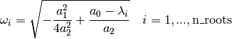
to the considered eigenvalue problem.
Parameters: - param (array_like) –
- l (numbers.Number) – Right boundary value of the domain
![[0,l]\ni z](../_images/math/a764cb846ff2a6542ce23c718f87a93572eeaf24.png) .
. - n_roots (int) – Amount of eigenfrequencies to be compute.
Returns: Return type: tuple –> two numpy.ndarrays of length n_roots
- param (array_like) –
- om (numbers.Number) – eigenfrequency
-
class
SecondOrderRobinEigenfunction(om, param, l, scale=1, max_der_order=2)[source]¶ Bases:
pyinduct.core.Function,pyinduct.eigenfunctions.SecondOrderEigenfunctionThis class provides an eigenfunction
to the eigenvalue
problem given by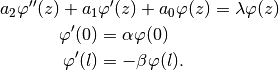
The eigenfrequency
must be provided (for example with the
eigfreq_eigval_hint()of this class).Parameters: - om (numbers.Number) – eigenfrequency
- param (array_like) –
- l (numbers.Number) – End of the domain .
- scale (numbers.Number) – Factor to scale the eigenfunctions (corresponds
to
 ).
). - max_der_order (int) – Number of derivative handles that are needed.
-
static
eigfreq_eigval_hint(param, l, n_roots, show_plot=False)[source]¶ Return the first n_roots eigenfrequencies
and eigenvalues .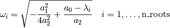
to the considered eigenvalue problem.
Parameters: - param (array_like) –
- l (numbers.Number) – Right boundary value of the domain .
- n_roots (int) – Amount of eigenfrequencies to compute.
- show_plot (bool) – Show a plot window of the characteristic equation.
Returns: ![\Big(\big[\omega_1, \dotsc, \omega_{\text{n\_roots}}\Big],
\Big[\lambda_1, \dotsc, \lambda_{\text{n\_roots}}\big]\Big)](../_images/math/5949c5f44f57cda1bd94664214f6aa7da120e324.png)
Return type: tuple –> booth tuple elements are numpy.ndarrays of length nroots
- param (array_like) –
- om (numbers.Number) – eigenfrequency
-
class
TransformedSecondOrderEigenfunction(target_eigenvalue, init_state_vector, dgl_coefficients, domain)[source]¶ Bases:
pyinduct.core.FunctionThis class provides an eigenfunction
to the eigenvalue
problem given by
where
 denotes an eigenvalue and
![z \in [z_0, \dotsc, z_n]](../_images/math/5cc91a2d01d5e7a94885ca3448322f0898e77d51.png) the domain.
the domain.Parameters: - target_eigenvalue (numbers.Number) –
- init_state_vector (array_like) –
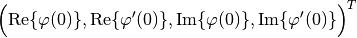
- dgl_coefficients (array_like) – Function handles
 .
. - domain (
Domain) – Spatial domain of the problem.
- target_eigenvalue (numbers.Number) –
-
class
AddMulFunction(function)[source]¶ Bases:
object(Temporary) Function class which can multiplied with scalars and added with functions. Only needed to compute the matrix (of scalars) vector (of functions) product in
FiniteTransformFunction. Will be no longer needed whenFunctionis overloaded with__add__and__mul__operator.Parameters: function (callable) –
-
class
LambdifiedSympyExpression(sympy_funcs, spat_symbol, spatial_domain)[source]¶ Bases:
pyinduct.core.FunctionThis class provides a
Function based on a
lambdified sympy expression. The sympy expressions for the function and it’s
spatial derivatives must be provided as the list sympy_funcs. The
expressions must be provided with increasing derivative order, starting with
order 0.Parameters: - sympy_funcs (array_like) – Sympy expressions for the function and the
derivatives:
 .
. - spat_symbol – Sympy symbol for the spatial variable
 .
. - spatial_domain (tuple) – Domain on which is defined
(e.g.:
spatial_domain=(0, 1)).
- sympy_funcs (array_like) – Sympy expressions for the function and the
derivatives:
-
class
FiniteTransformFunction(function, M, l, scale_func=None, nested_lambda=False)[source]¶ Bases:
pyinduct.core.FunctionThis class provides a transformed
Function through the transformation
 , with the function
vector
, with the function
vector  and with a given matrix
 . The operator
  denotes the
matrix (of scalars) vector (of functions) product. The interim result
denotes the
matrix (of scalars) vector (of functions) product. The interim result
 is a vector
of functions
![&\bar\xi_{1,j} = \bar x(jl_0 + z),
\qquad j=0,...,n-1, \quad l_0=l/n, \quad z\in[0,l_0] \\
&\bar\xi_{2,j} = \bar x(l - jl_0 + z).](../_images/math/89fb9250f3d46991da1f3ffdb0475aca70a8db34.png)
Finally, the provided function
is given through
 .
.Note
For a more extensive documentation see section 4.2 in:
- Wang, S. und F. Woittennek: Backstepping-Methode für parabolische Systeme mit punktförmigem inneren Eingriff. Automatisierungstechnik, 2015. http://dx.doi.org/10.1515/auto-2015-0023
Parameters: - function (callable) –
Function
 that will act as start for the generation of
 Functions
![&\bar\xi_{1,j} = x(z + jl_0),
\qquad j=0,...,n-1, \quad l_0=l/n, \quad z\in[0,l_0] \\
&\bar\xi_{2,j} = x(z + l - jl_0 ).](../_images/math/55a4b01866fd25fc2f76c54fb3ba3483a1d4f368.png)
The vector of functions
 will then be
constituted as follows:
will then be
constituted as follows:
- M (numpy.ndarray) – Matrix of
scalars.
- l (numbers.Number) – Length of the domain ().