General
-
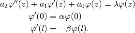
compute_rad_robin_eigenfrequencies(param, l, n_roots=10, show_plot=False)[source]¶ Return the first
n_rootseigenfrequencies (and eigenvalues
  )
)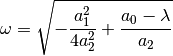
to the eigenvalue problem
Parameters: - param (array_like) –
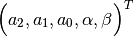
- l (numbers.Number) – Right boundary value of the domain
![[0,l]\ni z](../../_images/math/a764cb846ff2a6542ce23c718f87a93572eeaf24.png) .
. - n_roots (int) – Amount of eigenfrequencies to be compute.
- show_plot (bool) – A plot window of the characteristic equation appears
if it is
True.
Returns: ![\Big(\big[\omega_1,...,\omega_\text{n\_roots}\Big],
\Big[\lambda_1,...,\lambda_\text{n\_roots}\big]\Big)](../../_images/math/d8f5ce58efd7eca68255cb266f159f67c609d969.png)
Return type: tuple –> two numpy.ndarrays of length
nroots- param (array_like) –
-
eliminate_advection_term(param, domain_end)[source]¶ This method performs a transformation
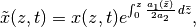
on the system, which eliminates the advection term
 from a
reaction-advection-diffusion equation of the type:
from a
reaction-advection-diffusion equation of the type:
The boundary can be given by robin

dirichlet

or mixed boundary conditions.
Parameters: - param (array_like) –
- domain_end (float) – upper bound of the spatial domain
Raises: TypeError– If is callable but no derivative handle is
- defined for it.
Returns: Parameters
the transformed system

and the corresponding boundary conditions (
 and/or
 set to None by dirichlet boundary condition).
Return type: SecondOrderOperator or tuple
- param (array_like) –
-
get_parabolic_dirichlet_weak_form(init_func_label, test_func_label, input_handle, param, spatial_domain)[source]¶ Return the weak formulation of a parabolic 2nd order system, using an inhomogeneous dirichlet boundary at both sides.
Parameters: - init_func_label (str) – Label of shape base to use.
- test_func_label (str) – Label of test base to use.
- input_handle (
SimulationInput) – Input. - param (tuple) – Parameters of the spatial operator.
- spatial_domain (#) – Spatial domain of the problem.
- spatial_domain – Spatial domain of the
- problem. (#) –
Returns: Weak form of the system.
Return type:
-
get_parabolic_robin_weak_form(shape_base_label, test_base_label, input_handle, param, spatial_domain, actuation_type_point=None)[source]¶ Parameters: - shape_base_label –
- test_base_label –
- input_handle –
- param –
- spatial_domain –
- actuation_type_point –
Returns:
-
get_in_domain_transformation_matrix(k1, k2, mode='n_plus_1')[source]¶ Returns the transformation matrix M. M is one part of a transformation
where x is the field variable of an interior point controlled parabolic system and y is the field variable of an boundary controlled parabolic system. T is a (Fredholm-) integral transformation (which can be approximated with M).
Parameters: - k1 –
- k2 –
- mode –
Available modes:
- ’n_plus_1’: M.shape = (n+1,n+1), w = (w(0),…,w(n))^T, w in {x,y}
- ‘2n’: M.shape = (2n,2n), w = (w(0),…,w(n),…,w(1))^T, w in {x,y}
Returns: Transformation matrix M.
Return type: numpy.array